
このページは、nAGライブラリのJupyterノートブックExampleの日本語翻訳版です。オリジナルのノートブックはインタラクティブに操作することができます。
nAGライブラリを使用した二次錐計画法(SOCP)によるポートフォリオ最適化のモデリング技法
このノートブックの正しいレンダリング
このノートブックでは、方程式と参照のためにlatex_envs
Jupyter拡張機能を使用しています。LaTeXがローカルのJupyterインストールで適切にレンダリングされない場合は、この拡張機能をインストールしていない可能性があります。詳細は
https://jupyter-contrib-nbextensions.readthedocs.io/en/latest/nbextensions/latex_envs/README.html
を参照してください。
また、このノートブックはGitHubでは適切にレンダリングされないため、GitHubで閲覧している場合は、PDF版を参照することをお勧めします。
nAGライブラリMark (27.1)以降のユーザーへの注意
nAGライブラリのMark \(27.1\)では、ユーザーが二次制約付き二次計画問題(QCQP)を簡単に定義できるよう、2つの新機能が追加されました。このノートブックのすべてのモデルは、再定式化や追加の労力なしで、より簡単に解くことができます。nAGライブラリMark \(27.1\)以降のユーザーは、QCQPに関するノートブックを参照することをお勧めします。
はじめに
二次錐計画法(SOCP)は、線形計画法(LP)を二次(ローレンツまたはアイスクリーム)錐で拡張した凸最適化です。解の探索領域は、アフィン線形多様体と二次錐のデカルト積の交差です。SOCPは、工学、制御理論、定量的金融から二次計画法やロバスト最適化まで、幅広い応用分野に現れます。その強力な性質により、金融最適化の重要なツールとなっています。内点法(IPM)は、理論的な多項式複雑性と実用的な性能により、SOCP問題を解くための最も一般的なアプローチです。
nAGは、Mark \(27\)で標準形式の大規模SOCP問題に対する内点法を導入しています: \[\begin{equation}\label{SOCP} \begin{array}{ll} \underset{x\in\Re^n}{\mbox{minimize}} & c^Tx\\[0.6ex] \mbox{subject to} & l_A\leq Ax\leq u_A,\\[0.6ex] & l_x\leq x\leq u_x,\\[0.6ex] & x\in{\cal K}, \end{array} \end{equation}\] ここで、\(A\in\Re^{m\times n}\)、\(l_A, u_A\in\Re^m\)、\(c, l_x, u_x\in\Re^n\)は問題データであり、\(\cal K={\cal K}^{n_1}\times\cdots\times{\cal K}^{n_r}\times\Re^{n_l}\)で、\({\cal K}^{n_i}\)は以下のように定義される二次錐または回転二次錐のいずれかです:
SOCPは、その柔軟性と多様性により、ポートフォリオ最適化で広く使用されています。様々な種類の制約を持つ多くの問題を扱うことができ、それらは(SOCP)と同等のSOCPに変換できます。詳細についてはを参照してください。この記事の残りの部分では、nAG Library for PythonのSOCPソルバーを使用して、ポートフォリオ最適化のための様々な実用的な制約を持つモデルを構築し解く方法を示します。
データ準備
2018年3月から2019年3月までのDJIAの30銘柄の日次価格を考えます。実際には、平均リターン\(r\)と共分散\(V\)の推定は多くの場合、簡単な作業ではありません。このノートブックでは、単純なサンプル推定を使用してこれらの値を推定します。
# 必要なライブラリをインポート
import pickle as pkl
import numpy as np
import matplotlib.pyplot as plt
# stock_price.plkから株価データを読み込む
# Stock_price: dict = ['close_price': [データ], 'date_index': [データ]]
stock_price = stock_price = pkl.load(open('./data/stock_price.pkl', 'rb'))
close_price = stock_price['close_price']
date_index = stock_price['date_index']# データのサイズ、m: 観測数、n: 株式数
m = len(date_index)
n = len(close_price)# 株価の終値をnumpy配列に抽出する
data = np.zeros(shape=(m, n))
i = 0
for stock in close_price:
data[:,i] = close_price[stock]
plt.plot(np.arange(m), data[:,i])
i += 1
# 終値をプロットする
plt.xlabel('Time (days)')
plt.ylabel('Closing price ($)')
plt.show()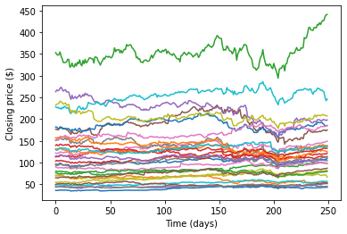
各銘柄 \(i\) について、まず \(j\) 日目の日次相対リターンを以下のように推定します: \[relative~return_{i,j} = \frac{closing~price_{i,j+1}-closing~price_{i,j}}{closing~price_{i,j}}.\]
# 相対リターン
rel_rtn = np.zeros(shape=(m-1, n))
for j in range(m-1):
    rel_rtn[j,:] = np.divide(data[j+1,:] - data[j,:], data[j,:])
# 相対リターンをプロット
for i in range(n):
    plt.plot(np.arange(m-1),rel_rtn[:,i])
plt.xlabel('Time (days)')
plt.ylabel('Relative return')
plt.show()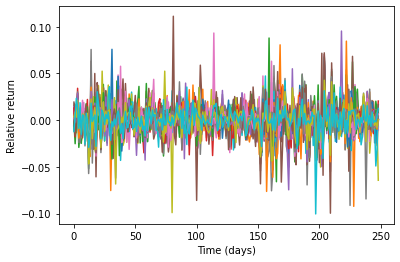
各株式の平均リターン \(r\) を得るために、相対リターンの各列の算術平均を単純に取り、その後、numpyを使用して共分散 \(V\) を推定します。
# 平均リターン
r = np.zeros(n)
r = rel_rtn.sum(axis=0)
r = r / (m-1)
# 共分散行列
V = np.cov(rel_rtn.T)
古典的な平均分散モデル
効率的フロンティア
ポートフォリオ管理の主要な目標の1つは、特定のリスク測定の下で一定水準のリターンを達成することです。ここでは、nAGライブラリを使用して、ロングオンリー制約(つまり、買い持ちのみで空売りは許可されない)を持つ古典的なマーコビッツモデルを解くことで、効率的フロンティアを構築する方法を示します: \[\begin{equation}\label{MV_model} \begin{array}{ll} \underset{x\in\Re^n}{\mbox{minimize}} & -r^Tx+\mu x^TVx\\[0.6ex] \mbox{subject to} & e^Tx = 1,\\[0.6ex] & x\geq0, \end{array} \end{equation}\] ここで、\(e\in\Re^n\)はすべて1のベクトルで、\(\mu\)はリターンとリスクのトレードオフを制御するスカラーです。\(\mu\)を0から特定の値まで変化させることで効率的フロンティアを構築できることに注意してください。
# nAGライブラリをインポートする
from naginterfaces.base import utils
from naginterfaces.library import opt
from naginterfaces.library import lapackeig
# 必要な数学ライブラリをインポート
import math as mt
import warnings as wn問題(MV_model)をSOCPを通じて解くには、それを標準形式(SOCP)に変換し、nAG SOCPソルバーにデータ\(A\)、\(l_A\)、\(u_A\)、\(c\)、\(l_x\)、\(u_x\)、および\(\cal K\)を与える必要があります。このモデリングプロセスはSOCPの使用に不可欠です。これらの再定式化テクニックに慣れることで、SOCPの最大限の力を引き出すことができるでしょう。
ソルバーが必要とするデータを管理するために、辞書構造を作成し維持することができます。
def model_init(n):
    """
    Initialize a dict to store the data that is used to feed nAG socp solver
    """
    model = {
#        変数の数
         'n': n,
#        制約条件の数
         'm': 0,
#        目的関数の係数
         'c': np.full(n, 0.0, float),
#        変数に対する境界制約
         'blx': np.full(n, -1.e20, float),
         'bux': np.full(n, 1.e20, float),
#        線形制約の係数とその境界
         'linear': {'bl': np.empty(0, float),
                    'bu': np.empty(0, float),
                    'irowa': np.empty(0, int),
                    'icola': np.empty(0, int),
                    'a': np.empty(0, float)},
#        円錐制約タイプと変数グループ
         'cone' : {'type': [],
                   'group': []}
         }
return modelデータモデルが完成したら、以下の関数を使用してnAG SOCP ソルバーにデータを供給することができます。
def set_nag(model):
    """
    Use data in model to feed nAG optimization suite to define problm
    """

#   問題ハンドルを作成する
    handle = opt.handle_init(model['n'])

#   目的関数を設定する
    opt.handle_set_linobj(handle, model['c'])

#   箱型制約を設定する
    opt.handle_set_simplebounds(handle, model['blx'], model['bux'])

#   線形制約を設定する
    opt.handle_set_linconstr(handle, model['linear']['bl'], model['linear']['bu'],
            model['linear']['irowa'], model['linear']['icola'], model['linear']['a'])

#   円錐制約を設定する
    i = 0
    while i<len(model['cone']['type']):
        opt.handle_set_group(handle,model['cone']['type'][i],
                             0, model['cone']['group'][i])
        i += 1

#   オプションを設定
    for option in [
            'Print Options = NO',
            'Print Level = 1',
            'Print File = -1',
            'SOCP Scaling = A'
    ]:
        opt.handle_opt_set(handle, option)

return handleそれでは、データをモデルに準備する方法に焦点を当てましょう。二次目的関数をモデルに追加するために、以下の変換が必要です。変数\(t\)を導入することで、 \[\begin{equation} \begin{array}{ll} \underset{x\in\Re^n}{\mbox{minimize}} & -r^Tx+\mu x^TVx \end{array} \end{equation}\] は以下と等価になることに注意してください \[\begin{equation}\label{e_1} \begin{array}{ll} \underset{x\in\Re^n}{\mbox{minimize}} & -r^Tx+t\\ \mbox{subject to} & \mu x^TVx\leq t \end{array} \end{equation}\] ただし、\(V\)は正半定値行列です。これで(e_1)の目的関数は線形となり、標準モデル(SOCP)に適合します。\(V=F^TF\)と因数分解することで、(e_1)の二次不等式を以下のように書き換えることができます \[\label{e_2} \mu\|Fx\|^2\leq t, \] ここで\(\|\cdot\|\)はユークリッドノルムです。\(y=Fx\)と\(s=\frac{1}{2\mu}\)を導入することで、(e_2)は以下のように書き換えられることに注意してください \[ \|y\|^2\leq 2st, \] これは錐制約(RSOC)と全く同じ形式です。したがって、問題(MV_model)の最終的なSOCP定式化は以下のようになります \[\begin{equation}\label{MV_model_trans} \begin{array}{ll} \underset{x\in\Re^n, y\in\Re^n, s\in\Re, t\in\Re}{\mbox{minimize}} & -r^Tx+t\\[0.6ex] \mbox{subject to} & e^Tx = 1,\\[0.6ex] & Fx - y = 0,\\ & s=\frac{1}{2\mu},\\ & x\geq0,\\ & (s,t,y)\in{\cal K}^{n+2}_r. \end{array} \end{equation}\] \(V\)の因数分解は、nAGライブラリを使用して以下のように行うことができます。
def factorize(V):
    """
    For any given positive semidefinite matrix V, factorize it V = F'*F where
    F is kxn matrix that is returned
    """
#   Vのサイズ
    n = V.shape[0]

#   注意: Vがスパース行列として入力される場合、スパース因子分解を使用することができます
    U, lamda = lapackeig.dsyevd('V', 'L', V)

#   正の固有値と対応する固有ベクトルを求める
    i = 0
    k = 0
    F = []

    while i<len(lamda):
        if lamda[i] > 0:
            F = np.append(F, mt.sqrt(lamda[i])*U[:,i])
            k += 1
        i += 1

    F = F.reshape((k, n))

    return F
以下のコードは一般的な二次目的関数 \[\begin{equation} \begin{array}{ll} \underset{x\in\Re^n}{\mbox{minimize}} & \frac{1}{2}x^TVx + q^Tx \end{array} \end{equation}\] をモデルに追加します。
def add_qobj(model, F, q=None):
    """
    Add quadratic objective defined as: 1/2 * x'Vx + q'x
    transformed to second order cone by adding artificial variables

    Parameters
    ----------
    model: a dict with structure:
        {
         'n': int,
         'm': int,
         'c': float numpy array,
         'blx': float numpy array,
         'bux': float numpy array,
         'linear': {'bl': float numpy array,
                    'bu': float numpy array,
                    'irowa': int numpy array,
                    'icola': int numpy array,
                    'a': float numpy array},
         'cone' : {'type': character list,
                   'group': nested list of int numpy arrays}
        }
    F: float 2d numpy array
        kxn dense matrix that V = F'*F where k is the rank of V
    q: float 1d numpy array
        n vector

    Returns
    -------
    model: modified structure of model

    Note: imput will not be checked
    """

#   Fの次元を取得する (kxn)
    k, n = F.shape

#   デフォルト q
    if q is None:
        q = np.zeros(n)

#   最新の問題サイズ
    m_up = model['m']
    n_up = model['n']

#   その後、k + 2個のさらなる変数を以下と共に加える必要があります
#   k + 1個の線形制約と1つの回転円錐制約
#   モデルを拡大する
    model['n'] = model['n'] + k + 2
    model['m'] = model['m'] + k + 1

#   目的関数内のcを初期化する
#   変数の順序は [x, t, y, s] です
    model['c'][0:n] = q
    model['c'] = np.append(model['c'], np.zeros(k+2))
    model['c'][n_up] = 1.0

#   xの境界を拡大し、新たに追加されたk+2個の変数に無限大の境界を追加する
    model['blx'] = np.append(model['blx'], np.full(k+2, -1.e20, dtype=float))
    model['bux'] = np.append(model['bux'], np.full(k+2, 1.e20, dtype=float))

#   線形制約の拡大
#   Fの疎パターンを取得する
    row, col = np.nonzero(F)
    val = F[row, col]

#   1ベースに変換し、行を m だけ下に移動する
    row = row + 1 + m_up
    col = col + 1
#   yとtとsの係数を既存の線形係数Aに追加する
#   結果は
#                  [A, 0,  0, 0;
#                   F, 0, -I, 0;
#                   0, 0,  0, 1]
    row = np.append(row, np.arange(m_up+1, m_up+k+1+1))
    col = np.append(col, np.arange(n_up+2, n_up+k+1+1+1))
    val = np.append(val, np.append(np.full(k, -1.0, dtype=float), 1.0))
    model['linear']['irowa'] = np.append(model['linear']['irowa'], row)
    model['linear']['icola'] = np.append(model['linear']['icola'], col)
    model['linear']['a'] = np.append(model['linear']['a'], val)

    model['linear']['bl'] = np.append(model['linear']['bl'],
                                      np.append(np.zeros(k), 1.0))
    model['linear']['bu'] = np.append(model['linear']['bu'],
                                      np.append(np.zeros(k), 1.0))

#   円錐制約の拡大
    model['cone']['type'].extend('R')
    group = np.zeros(k+2, dtype=int)
    group[0] = n_up + 1
    group[1] = n_up + 1 + k + 1
    group[2:] = np.arange(n_up+2, n_up+k+1+1)
    model['cone']['group'].append(group)

return model(MV_model)の目的関数が追加されたら、以下の関数を使用して長期のみの制約を追加することができます\[e^Tx=1~\mbox{and}~x\geq0.\]
def add_longonlycon(model, n, b=None):
    """
    Add long-only constraint to model
    If no b (benchmark) presents, add sum(x) = 1, x >= 0
    If b presents, add sum(x) = 0, x + b >= 0
    """
#   最新の問題サイズ
    m = model['m']

#   制約条件の数が1増加しました
    model['m'] = model['m'] + 1

#   境界制約: x >=0 または x >= -b
    if b is not None:
        model['blx'][0:n] = -b
    else:
        model['blx'][0:n] = np.zeros(n)

#   線形制約: e'x = 1 または e'x = 0
    if b is not None:
        model['linear']['bl'] = np.append(model['linear']['bl'],
                                          np.full(1, 0.0, dtype=float))
        model['linear']['bu'] = np.append(model['linear']['bu'],
                                          np.full(1, 0.0, dtype=float))
    else:
        model['linear']['bl'] = np.append(model['linear']['bl'],
                                          np.full(1, 1.0, dtype=float))
        model['linear']['bu'] = np.append(model['linear']['bu'],
                                          np.full(1, 1.0, dtype=float))

    model['linear']['irowa'] = np.append(model['linear']['irowa'],
                                         np.full(n, m+1, dtype=int))
    model['linear']['icola'] = np.append(model['linear']['icola'],
                                         np.arange(1, n+1))
    model['linear']['a'] = np.append(model['linear']['a'],
                                     np.full(n, 1.0, dtype=float))

    return model
上記の関数を使用することで、以下のように効率的フロンティアを簡単に構築できます。
def ef_lo_basic(n, r, V, step=None):
    """
    Basic model to build efficient frontier with long-only constraint
    by solving:
        min -r'*x + mu * x'Vx
        s.t. e'x = 1, x >= 0
    Parameters
    ----------
    n: number of assets
    r: expected return
    V: covariance matrix
    step: define smoothness of the curve of efficient frontier,
          mu would be generated from [0, 2000] with step in default

    Output:
    -------
    risk: a vector of risk sqrt(x'Vx) with repect to certain mu
    rtn: a vector of expected return r'x with repect to certain mu
    """

#   オプション引数を設定する
    if step is None:
        step = 2001

#   一度だけVを因数分解し、残りのコードでその因数分解を使用する
#   密行列 V = U*Diag(lamda)*U' の固有値分解を行い、V = F'*F を得る
    F = factorize(V)

    risk = np.empty(0, float)
    rtn = np.empty(0, float)

    for mu in np.linspace(0.0, 2000.0, step):
#       モデルを構築するためのデータ構造を初期化する
        model = model_init(n)

#       2次目的関数
        muf = F * mt.sqrt(2.0*mu)

        model = add_qobj(model, muf, -r)

#       売り持ちなし制約を追加
        model = add_longonlycon(model, n)

#       モデルを使用してnAG socpソルバーに供給します
        handle = set_nag(model)

#       内点法SOCPソルバーを呼び出す
#       警告をミュートし、警告からの結果をカウントしない
        wn.simplefilter('error', utils.NagAlgorithmicWarning)
        try:
            slt = opt.handle_solve_socp_ipm(handle)

#           ポートフォリオのリスクとリターンを計算する
            risk = np.append(risk, mt.sqrt(slt.x[0:n].dot(V.dot(slt.x[0:n]))))
            rtn = np.append(rtn, r.dot(slt.x[0:n]))
        except utils.NagAlgorithmicWarning:
            pass

#       ハンドルを破棄する:
        opt.handle_free(handle)

    return risk, rtn
# 効率的フロンティアを構築し、結果をプロットする
ab_risk, ab_rtn = ef_lo_basic(n, r, V, 500)
plt.plot(ab_risk*100.0, ab_rtn*100.0)
plt.ylabel('Total Expected Return (%)')
plt.xlabel('Absolute Risk (%)')
plt.show()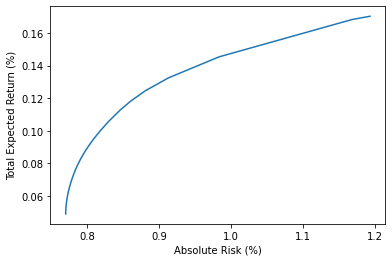
シャープレシオの最大化
シャープレシオは、ポートフォリオのリターンとポートフォリオの超過リターンの標準偏差の比率として定義されます。通常、ポートフォリオの効率性を測定するために使用されます。最も効率的なポートフォリオを見つけることは、以下の最適化問題を解くことと同等です。 \[\begin{equation}\label{sr_model} \begin{array}{ll} \underset{x\in\Re^n}{\mbox{minimize}} & \frac{\sqrt{x^TVx}}{r^Tx}\\[0.6ex] \mbox{subject to} & e^Tx = 1,\\[0.6ex] & x\geq0. \end{array} \end{equation}\] \(x\)を\(\frac{y}{\lambda}, \lambda\gt0\)で置き換えることで、モデル(sr_model)は以下と同等になります: \[\begin{equation}\label{sr_model_eq} \begin{array}{ll} \underset{y\in\Re^n, \lambda\in\Re}{\mbox{minimize}} & y^TVy\\[0.6ex] \mbox{subject to} & e^Ty = \lambda,\\[0.6ex] & r^Ty=1, \\ & y\geq0, \\ & \lambda\geq0. \end{array} \end{equation}\] 問題(sr_model_eq)は、二次目的関数と線形制約を持つという点で問題(MV_model)と類似しています。線形制約の定義を除いて再定式化がほぼ同じであるため、上記の関数のほとんどを再利用できます。そのために、以下の関数が必要です。
def add_sr_lincon(model, r, n):
    """
    Add linear constraints for Sharpe ratio problem
    e'y = lamda, y >= 0, r'y = 1, lamda >= 0
    Enlarge model by 1 more variable lamda
    Return: model and index of lambda in the final result, need it to
            reconstruct the original solution
    """
#   最新の問題サイズ
    m_up = model['m']
    n_up = model['n']

#   さらに1つの変数と2つの線形制約を追加する
    model['n'] = model['n'] + 1
    model['m'] = model['m'] + 2

#   パラメータ0.0でcを拡大する
    model['c'] = np.append(model['c'], 0.0)

#   yの境界制約
    model['blx'][0:n] = np.zeros(n)

#   ラムダに境界制約を設定する
    model['blx'] = np.append(model['blx'], 0.0)
    model['bux'] = np.append(model['bux'], 1.e20)

#   e'y = lamda を追加
    row = np.full(n+1, m_up+1, dtype=int)
    col = np.append(np.arange(1, n+1), n_up+1)
    val = np.append(np.full(n, 1.0, dtype=float), -1.0)

#   y = 1 を追加
    row = np.append(row, np.full(n, m_up+2, dtype=int))
    col = np.append(col, np.arange(1, n+1))
    val = np.append(val, r)

#   モデルを更新
    model['linear']['irowa'] = np.append(model['linear']['irowa'], row)
    model['linear']['icola'] = np.append(model['linear']['icola'], col)
    model['linear']['a'] = np.append(model['linear']['a'], val)

#   線形制約の境界
    model['linear']['bl'] = np.append(model['linear']['bl'],
                                      np.append(np.zeros(1), 1.0))
    model['linear']['bu'] = np.append(model['linear']['bu'],
                                      np.append(np.zeros(1), 1.0))

return model, n_upこれで以下のようにnAG SOCPソルバーを呼び出すことができます。
def sr_lo_basic(n, r, V):
    """
    Basic model to calculate efficient portfolio that maximize the Sharpe ratio
    min y'Vy
    s.t. e'y = lamda, y >= 0, r'y = 1, lamda >= 0
    Return efficient portfolio y/lamda and corresponding risk and return
    """
#   一度だけVを因数分解し、残りのコードでその因数分解を使用する
#   密行列 V = U*Diag(lamda)*U' の固有値分解を行い、V = F'*F を得る
    F = factorize(V)

#   モデルを構築するためのデータ構造を初期化する
    model = model_init(n)

#   2次目的関数
    muf = F * mt.sqrt(2.0)

    model = add_qobj(model, muf)

#   線形制約を追加する
    model, lamda_idx = add_sr_lincon(model, r, n)

#   モデルを使用してnAG socpソルバーに供給します
    handle = set_nag(model)

#   内点法SOCPソルバーを呼び出す
    slt = opt.handle_solve_socp_ipm(handle)

    sr_risk = mt.sqrt(slt.x[0:n].dot(V.dot(slt.x[0:n])))/slt.x[lamda_idx]
    sr_rtn = r.dot(slt.x[0:n])/slt.x[lamda_idx]

    return sr_risk, sr_rtn, slt.x[0:n]/slt.x[lamda_idx]
# 最も効率的なポートフォリオを計算し、結果をプロットします。
sr_risk, sr_rtn, sr_x = sr_lo_basic(n, r, V)
plt.plot(ab_risk*100.0, ab_rtn*100.0, label='Efficient frontier')
plt.plot([sr_risk*100], [sr_rtn*100], 'rs',
label='Portfolio with maximum Sharpe ratio')
plt.plot([sr_risk*100, 0.0], [sr_rtn*100, 0.0], 'r-', label='Capital market line')
plt.axis([min(ab_risk*100), max(ab_risk*100), min(ab_rtn*100), max(ab_rtn*100)])
plt.ylabel('Total Expected Return (%)')
plt.xlabel('Absolute Risk (%)')
plt.legend()
plt.show()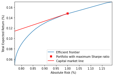
トラッキングエラー制約付きポートフォリオ最適化
ベンチマークを上回る際に不必要なリスクを取ることを避けるため、投資家は一般的にアクティブポートフォリオのベンチマークからの乖離の変動性に制限を設けます。これはトラッキングエラー変動性(TEV)としても知られています 。超過リターン空間で効率的フロンティアを構築するモデルは以下の通りです: \[\begin{equation}\label{er_tev} \begin{array}{ll} \underset{x\in\Re^n}{\mbox{maximize}} & r^Tx\\ \mbox{subject to} & e^Tx = 0,\\ & x^TVx\leq tev, \end{array} \end{equation}\] ここで \(tev\) はトラッキングエラーの制限です。Roll は、問題 (er_tev) がベンチマークと全く無関係であり、アクティブポートフォリオが体系的にベンチマークよりも高いリスクを持ち、最適ではないという好ましくない結果につながると指摘しました。そのため、本セクションでは絶対リスクを考慮したより高度なモデルを以下のように解きます。 \[\begin{equation}\label{tev_model} \begin{array}{ll} \underset{x\in\Re^n}{\mbox{minimize}} & -r^Tx+\mu (x+b)^TV(x+b)\\ \mbox{subject to} & e^Tx = 0,\\ & x^TVx\leq tev,\\ & x+b\geq0, \end{array} \end{equation}\] ここで \(b\) はベンチマークポートフォリオです。このデモンストレーションでは、これは人工的に生成されています。ここでは、デモンストレーションの目的で、TEVと絶対リスク測定に同じ共分散行列 \(V\) を使用していることに注意してください。実際には、異なる市場から異なる共分散行列を使用することができます。
# 効率的ポートフォリオからベンチマークポートフォリオを生成する
# シャープレシオを最大化する
# xを摂動させる
b = sr_x + 1.e-1
# bを正規化する
b = b/sum(b)

# ベンチマークにおけるリスクとリターンを計算する
b_risk = mt.sqrt(b.dot(V.dot(b)))
b_rtn = r.dot(b)問題(MV_model)と同様に、(tev_model)の目的関数は二次式であるため、\(add\_qobj()\)を使用してモデルに追加できることに注意してください。しかし、問題(tev_model)には二次制約があり、これは二次制約付き二次計画問題(QCQP)となります。(e_1)の制約の変換と同様の手順に従って、一般的な二次制約を繰り返し追加するために再利用可能な関数を作成することができます。
def add_qcon(model, F, q=None, r=None):
    """
    Add quadratic contraint defined as: 1/2 * x'Vx + q'x + r <= 0,
    which is equivalent to t + q'x + r = 0, 1/2 * x'Vx <= t,
    transformed to second order cone by adding artificial variables

    Parameters
    ----------
    model: a dict with structure:
        {
         'n': int,
         'm': int,
         'c': float numpy array,
         'blx': float numpy array,
         'bux': float numpy array,
         'linear': {'bl': float numpy array,
                    'bu': float numpy array,
                    'irowa': int numpy array,
                    'icola': int numpy array,
                    'a': float numpy array},
         'cone' : {'type': character list,
                   'group': nested list of int numpy arrays}
        }
    F: float 2d numpy array
        kxn dense matrix that V = F'*F where k is the rank of V

    q: float 1d numpy array
        n vector

    r: float scalar

    Returns
    -------
    model: modified structure of model

    Note: imput will not be checked
    """
#   デフォルトパラメータ
    if r is None:
        r = 0.0

#   Fの次元を取得する (kxn)
    k, n = F.shape

#   最新の問題サイズ
    m_up = model['m']
    n_up = model['n']

#   その後、k + 2個のさらなる変数を以下と共に加える必要があります
#   k + 2個の線形制約と1つの回転円錐制約
#   モデルを拡大する
    model['n'] = model['n'] + k + 2
    model['m'] = model['m'] + k + 2

#   追加されたすべての補助変数は目的関数に関与しない
#   したがって、目的関数における彼らの係数はすべてゼロです。
    model['c'] = np.append(model['c'], np.zeros(k+2))

#   xの境界を拡大し、新たに追加されたk+2個の変数に無限大の境界を追加する
    model['blx'] = np.append(model['blx'], np.full(k+2, -1.e20, dtype=float))
    model['bux'] = np.append(model['bux'], np.full(k+2, 1.e20, dtype=float))

#   線形制約の拡大
    row, col = np.nonzero(F)
    val = F[row, col]

#   1ベースに変換し、行を m_up 分下に移動する
#   Fx = y と s = 1 を加える
#   [x,t,y,s]
    row = row + 1 + m_up
    col = col + 1
    row = np.append(np.append(row, np.arange(m_up+1, m_up+k+1+1)), m_up+k+1+1)
    col = np.append(np.append(col, np.arange(n_up+2, n_up+k+1+1+1)), n_up+1)
    val = np.append(np.append(val, np.append(np.full(k, -1.0,
                                                     dtype=float), 1.0)), 1.0)
    model['linear']['irowa'] = np.append(model['linear']['irowa'], row)
    model['linear']['icola'] = np.append(model['linear']['icola'], col)
    model['linear']['a'] = np.append(model['linear']['a'], val)

    model['linear']['bl'] = np.append(np.append(model['linear']['bl'],
                                                np.append(np.zeros(k), 1.0)), -r)
    model['linear']['bu'] = np.append(np.append(model['linear']['bu'],
                                                np.append(np.zeros(k), 1.0)), -r)

#   t + q'x + r = 0 を加える
    if q is not None:
        model['linear']['irowa'] = np.append(model['linear']['irowa'],
                                             np.full(n, m_up+k+2, dtype=int))
        model['linear']['icola'] = np.append(model['linear']['icola'],
                                             np.arange(1, n+1))
        model['linear']['a'] = np.append(model['linear']['a'], q)

#   円錐制約の拡大
    model['cone']['type'].extend('R')
    group = np.zeros(k+2, dtype=int)
    group[0] = n_up + 1
    group[1] = n_up + 1 + k + 1
    group[2:] = np.arange(n_up+2, n_up+k+1+1)
    model['cone']['group'].append(group)

    return model
上記の関数を使用することで、以下のようにTEV制約付きの効率的フロンティアを簡単に構築できます。
def tev_lo(n, r, V, b, tev, step=None):
    """
    TEV contrained portforlio optimization with absolute risk taken into
    consideration by solving:
    min -r'y + mu*(b+y)'V(b+y)
    s.t. sum(y) = 0, y+b >=o, y'Vy <= tev
    """
#   オプション引数の設定
    if step is None:
        step = 2001

#   一度だけVを因数分解し、残りのコードでその因数分解を使用する
#   密行列 V = U*Diag(lamda)*U' の固有値分解を行い、V = F'*F を得る
    F = factorize(V)

    risk = np.empty(0, float)
    rtn = np.empty(0, float)

    for mu in np.linspace(0.0, 2000.0, step):
#       モデルを構築するためのデータ構造を初期化する
        model = model_init(n)

#       売り持ちなし制約を追加
        model = add_longonlycon(model, n, b)

#       2次目的関数
        muf = F * mt.sqrt(2.0*mu)
        mur = 2.0*mu*V.dot(b) - r

        model = add_qobj(model, muf, mur)

#       二次制約 y'Vy <= tev を追加
        F_hf = F * mt.sqrt(2.0)
        model = add_qcon(model, F_hf, r=-tev)

#       モデルを使用してnAG socpソルバーに供給します
        handle = set_nag(model)

#       内点法SOCPソルバーを呼び出す
#       警告を無効にし、警告からの結果をカウントしない
        wn.simplefilter('error', utils.NagAlgorithmicWarning)
        try:
            slt = opt.handle_solve_socp_ipm(handle)

# ポートフォリオのリスクとリターンを計算する
            risk = np.append(risk, mt.sqrt((slt.x[0:n]+b).dot(V.dot(slt.x[0:n]+b))))
            rtn = np.append(rtn, r.dot(slt.x[0:n]+b))
        except utils.NagAlgorithmicWarning:
            pass

#       ハンドルを破棄する:
        opt.handle_free(handle)

    return risk, rtn
# トラッキングエラーの制限を設定する
tev = 0.000002
# モデルを解く
tev_risk, tev_rtn = tev_lo(n, r, V, b, tev, step=500)
# 結果をプロットする
plt.figure(figsize=(7.5, 5.5))
plt.plot(ab_risk*100.0, ab_rtn*100.0, label='Classic efficient frontier')
plt.plot([sr_risk*100], [sr_rtn*100], 'rs',
label='Portfolio with maximum Sharpe ratio')
plt.plot([sr_risk*100, 0.0], [sr_rtn*100, 0.0], 'r-', label='Capital market line')
plt.plot(b_risk*100, b_rtn*100, 'r*', label='Benchmark portfolio')
plt.plot(tev_risk*100.0, tev_rtn*100.0, 'seagreen',
label='Efficient frontier with tev constraint')
plt.axis([min(ab_risk*100), max(ab_risk*100), min(tev_rtn*100), max(ab_rtn*100)])
plt.ylabel('Total Expected Return (%)')
plt.xlabel('Absolute Risk (%)')
plt.legend()
plt.show()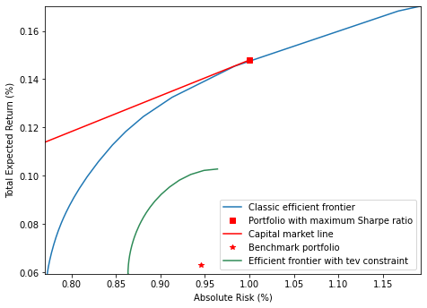
結論
このノートブックでは、ポートフォリオ最適化におけるさまざまなモデルを解くためにnAGライブラリを使用する方法を示しました。上記で言及した関数のいくつかを使用して、すぐに独自のモデルを構築し始めることができます。SOCPの汎用性は、ここで言及したモデルだけに限定されないことを指摘する価値があります。それはさらに多くの問題と制約をカバーしています。例えば、DeMiguelらはノルム制約付きのポートフォリオ最適化について議論しており、これは容易にSOCP問題に変換できます。SOCPソルバーに関するnAGライブラリのドキュメントとを参照してください。
参考文献
[1] Alizadeh Farid and Goldfarb Donald, ``Second-order cone programming’’, Mathematical programming, vol. 95, number 1, pp. 3–51, 2003.
[2] Lobo Miguel Sousa, Vandenberghe Lieven, Boyd Stephen et al., ``Applications of second-order cone programming’’, Linear algebra and its applications, vol. 284, number 1-3, pp. 193–228, 1998.
[3] Jorion Philippe, ``Portfolio optimization with tracking-error constraints’’, Financial Analysts Journal, vol. 59, number 5, pp. 70–82, 2003.
[4] Roll Richard, ``A mean/variance analysis of tracking error’’, The Journal of Portfolio Management, vol. 18, number 4, pp. 13–22, 1992.
[5] DeMiguel Victor, Garlappi Lorenzo, Nogales Francisco J et al., ``A generalized approach to portfolio optimization: Improving performance by constraining portfolio norms’’, Management science, vol. 55, number 5, pp. 798–812, 2009.
[6] Numerical Algorithms Group, ``nAG documentation’’, 2019. online